Rev. FCA UNCuyo | 2026 | 58(1) | ISSN 1853-8665
Natural resources and environment
https://doi.org/10.48162/rev.39.210
Climatic Normals in Chacras de Coria. Evolution of Air Temperature for the 1959-2020 Period
Normales climáticas de Chacras de Coria. La evolución de la temperatura del aire para el período 1959-2020
Adriana Inés Caretta 1,
Nora Beatriz Martinengo 1
1 Universidad Nacional de Cuyo. Facultad de Ciencias Agrarias. Almirante Brown 500. Chacras de Coria. M5528AHB. Mendoza. Argentina.
* cflores@fca.uncu.edu.ar
Abstract
Air temperature data registered from 1959 to 2020 by the Chacras de Coria meteorological station (32°59' S Lat.; 68°52' W Long.) were analyzed to characterize the site and identify trends considering the climate change scenario. We ensured quality and homogeneity of the time series following the procedures of the Standard World Meteorological Organization, calculating reference (1961-1990) and regulatory (1991-2020) climatological normals. The ClimPACT package detected trends in temperature-related indices, including extreme values, daily thermal amplitude, and degree days. The results reveal that the 1991-2020 period was 0.6°C warmer than 1961-1990. Significant increases were observed in average minimum (0.12°C/decade) and average maximum (0.20°C/decade) temperatures. Extreme minimum and maximum temperatures also increased by 0.11°C/decade and 0.33°C/decade, respectively, resulting in fewer cold nights (-0.49%/decade) and more hot days (1.6%/decade). Daily temperature ranges increased by 0.11°C/decade, and degree days by 52 DD/decade. These findings are consistent with global warming evidence. A corrected and homogenized database spanning over 60 years is available for future climatological studies.
Keywords: climatology, climate change, ClimPACT
Resumen
Se analizaron datos de temperatura del aire (1959-2020) de la estación meteorológica Chacras de Coria (32°59' Lat. S; 68°52' Long. O) para caracterizar el sitio e identificar tendencias bajo el escenario de Calentamiento Global y Cambio Climático. Se aplicaron procedimientos estándar de la Organización Meteorológica Mundial para asegurar la calidad y homogeneidad de las series temporales, calculando normales climatológicas de referencia (1961-1990) y regulatorias (1991-2020). Se utilizó el paquete ClimPACT para detectar tendencias en índices asociados a la temperatura, incluyendo valores extremos, amplitud térmica diaria y Grados Día. Los resultados revelan que el período 1991-2020 fue 0,6°C más cálido que 1961-1990. Se observaron incrementos significativos en las temperaturas mínimas promedio (0,12°C/década) y máximas promedio (0,20°C/década). Los valores extremos de temperaturas mínimas y máximas también aumentaron a razón de 0,11°C/década y 0,33°C/década respectivamente, lo que se tradujo en menos noches frías (-0,49%/década) y más días calurosos (1,6%/década). La amplitud térmica diaria creció 0,11°C/década, y los Grados Día en 52 GD/década. Estos hallazgos concuerdan con la evidencia global de calentamiento. Una base de datos de más de 60 años, corregida y homogeneizada, está disponible para futuros estudios climatológicos.
Palabras clave: climatología, cambio climático, ClimPACT
Originales: Recepción: 19/03/2025 - Aceptación: 19/12/2025
Introduction
Since 1959, the Chacras de Coria weather station located at 32°59' S. Lat.; 68°52' W. Long. (Facultad de Ciencias Agrarias - Universidad Nacional de Cuyo) has generated a rich heritage of high-quality meteorological data. This allowed us to establish climatological normals and calculate indices to analyze the evolution of Climatic Elements (CE), such as air temperatura and precipitation, which are crucial for understanding Climate Change (CC). Chacras de Coria is strategically located within the Mendoza River oasis, an area recently zoned under edaphoclimatic criteria as a region of high variability, where this site is part of one of the highland zones characterized by a warm climate and cold nights (Córdoba et al., 2025).
Climate Change refers to a statistically significant variation in the climate state. Climate Change can be caused by natural internal processes or external forcing. The latter are persistent anthropogenic changes in the atmospheric composition or land use. Thus, the increasing Greenhouse Gas (GHG) emissions generate heterogeneous impacts at the space-time scale. Changes observed from these situations become evident in the CE (9).
Globally, each successive decade has been warmer since 1990. Historical records indicate that the 2011-2020 decade was the warmest, with significant margins for both land and ocean temperatures. These temperature increases, along with sea acidification, level rise, ice masses loss, and more intense and frequent extreme events, are related to anthropogenic CC, especially linked to higher GHG concentrations (24).
This study calculated air temperature normals and investigated this CE in Chacras de Coria during the 1959-2020 period, characterizing this site and detecting trends.
Materials and Methods
Daily maximum and minimum air temperature values from January 1st, 1959, to December 31st, 2020, were used. Observations were made daily at 9:00, 15:00, and 21:00 h local time. The data was analyzed using the ClimPACT package. This package provides the frequency, duration, and magnitude of climate extremes relevant to agriculture and food security, health, and water resources. Such indices, designed to track heat waves, droughts, and precipitation extremes, are monthly and annually available. ClimPACT uses historical daily values of maximum and minimum temperature and daily precipitation to calculate over 60 different climate indices (4, 20).
Climate data is considered homogeneous when all serial fluctuations express real CE variability. Data are typically assumed free of instrumentation, coding or processing errors. However, meteorological and climatological data are usually heterogeneous and erratic. These errors can be systematic, affecting a complete set of observations, or random, like the differences in parallax between observers reading a mercury barometer. These are known as over- or under-error observations and can be independent or correlated. Independent errors in consecutive observations are considered random, while dependent errors are correlated from one observation to the next (23). Therefore, we evaluated and homogenized the climatic normals and proposed indices.
Data Quality Evaluation
Quality evaluation verifies that the reported data is representative and not contaminated by unrelated factors (23). This evaluation is performed before testing homogenization, since outliers can affect this latter process.
The 1961-1990 data were established as the base period as suggested by the WMO, considered the standard reference period for long-term climate change assessments. These years allow the user to calculate percentile thresholds (21).
ClimPACT reports outlier data based on interquartile ranges (IQR) defined as the difference between the 75th and 25th percentiles. In this study, outliers were defined as those values 3x IQR above p75 or below p25. Using the IQR to identify outliers avoids affecting the process by larger outliers, making a single evaluation process sufficient (4).
Histograms of decimal values also helped to identify rounding biases. Other anomalies addressed were, (i) events of 4 or more consecutive equal values of minimum and maximum temperatures, (ii) repeated dates, (iii) values over 50°C, (iv) dates on which maximum and minimum temperature differences with the previous day were 20°C or more, (v) dates when maximum temperature was lower than minimum temperature and (vi) number of missing values for each variable and year. Incorrect values were amended and recorded in a change log file after consulting the original meteorological logs. With a corrected database, a second data quality analysis process reviewed the generated files, assuring data rigor. Finally, homogenization tests were executed.
Homogeneity
Climate time series often exhibit spurious or “non-climatic” jumps as well as gradual modifications due to changes in station location, environment, exposure, instrumentation, or observing practices. These heterogeneities can seriously affect extreme values. Therefore, station historical metadata is crucial for solving these problems (25).
A reliable analysis of a climate time series relies on data consistency over time. This need is addressed by statistically testing data homogeneity and defining a consequent homogenization process. Considering daily data is highly variable compared to monthly or annual data, adjusting homogeneity can be arduous. In a homogeneity test, the null hypothesis considers the series analysed is homogeneous, while the alternative hypothesis considers it presents, at least, one change point (22). We tested homogeneity with the RHtestsV4 software based on the RHtestsV3 software package with the addition of quantile matching adjustments estimated with reference series (19).
Methods based on penalized maximum t-test (PMT) or F (PMF) can identify and fit multiple change points in a time series. While the PMT test uses reference stations required for homogeneity analysis, the PMF test can be used as an absolute method when no neighbouring stations can be used in the comparison, as in this study (17, 18).
For the homogenization analysis, we used the corrected file, previously transformed to fit the RHtestsV4 package, according to the quality control criteria already explained. This file was loaded with the requested parameters, including the missing data code and confidence level.
Climatological Normals
Considering the rapid pace of climate change and the need for up-to-date information for operational purposes, at the 17th World Meteorological Congress in 2015, the WMO introduced a novel approach to 30-year data periods. The standard climatological normal shifted from non-overlapping 30-year periods (1931-1960, 1961-1990, 1991-2020) to more recent 30-year periods beginning with a year ending in 1 and ending with a year finishing in 0. The period from 1961 to 1990 was retained as normal reference for long-term climate change assessments (21). We calculated the climatological normals for 1961-1990 (reference normal) and 1991-2020. The new approach now considers series that partially overlap and are updated every 10 years (2001-2030, 2011-2040, 2021-2050).
Due to the COVID-19 pandemic restrictions, 2020 data presented some discontinuities. However, the WMO concluded that a random distribution of missing days over a month generated 95% confidence interval corresponding, on average, to 11% of the standard deviation of the underlying daily values of 5 missing days, and 17% of the standard deviation of 10 days missing. This is equivalent, for example, to a few tenths of a degree Celsius for typical standard deviation values, considering daily maximum and minimum temperatures. However, when a substantial number of missing days are consecutive, additional uncertainty arises, given certain autocorrelation in most daily meteorological parameters (21).
A monthly value associated with the average of the daily values of a particular month was not calculated when any of the following criteria were met: (i) observations were missing for 11 or more days in a month or (ii) observations were missing for five or more consecutive days in the month. Likewise, a normal or average for a given month considered at least 24 of the 30 years, that is, at least 80% of the years averaging a period (21, 23). Furthermore, a remaining “suspicious or incorrect” value after undergoing the control process was considered missing within the series.
After data quality and homogeneity tests, the primary climatological parameters were obtained using InfoStat (2020).
The Indexes
ClimPACT provides 60 standardized indices that compare results across periods, regions, and different source data sets. Trends calculated by ClimPACT are based on Sen's slope (15), a nonparametric test, and reflect the median slope of all ordered pairs in a data set. Since it is less affected by outliers, it is also more appropriate for calculating trends in extreme values, such as those from climatic elements, compared to other common trend estimators like least squares. The 95% confidence intervals are calculated for the slope, along with lower and upper limits (4).
The evaluated indices were: (i) TNn: minimum temperature in a month (“temperature of the coldest night in the month”) (°C); (ii) TNm: average daily minimum temperature (°C); (iii) TMm: average daily temperature (°C); (iv) TXm: average daily maximum temperature (°C); (v) TXx: maximum temperature in the month (“temperature of the hottest day”) (°C); (vi) TN10p: percentage of days in which the minimum temperature is below the 10th percentile ("percentage of days with cold night temperatures", %); (vii) TX90p: percentage of days where the maximum temperature is above the 90th percentile ("percentage of days with hot daytime temperatures", %); (viii) DTR: average difference between daily maximum temperatura and daily minimum temperature ("daily average thermal amplitude", °C); (ix) GDDgrow10: Grow Degree Days (Lower Developmental Threshold = 10°C); and (x) FD: number of days with frost (number of days in which the minimum temperature is equal or below 0°C).
Results and Discussion
Our results did not present change points for a confidence level of 0.99; therefore, the series was considered homogeneous.
Climatological Normals
Tables 1 and 2, show Mean daily air temperatures (TMm) and Standard Deviations (S.D.) for 1961-1990 and 1991-2020.
Table 1. Mean daily air temperatures (TMm) and Standard Deviations (S.D.) (°C) (1961-1990).
Tabla 1. Medias diarias (TMm) y Desviaciones Estándar (D.E.) (°C) (1961-1990).
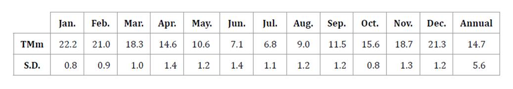
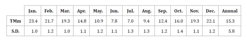
Table 2. Mean daily air temperatures (TMm) and Standard Deviations (S.D.) (°C) (1991-2020).
Tabla 2. Medias diarias (TMm) y Desviaciones Estándar (D.E.) (°C) (1991-2020).
Tables 3 and 4, show TNm and TNn values and their date of occurrence for 1961-1990 and 1991-2020.
Table 3. TNm and TNn values and their date of occurrence (°C) (1961-1990).
Tabla 3. Valores de TNm y TNn y su fecha de ocurrencia (°C) (1961-1990).
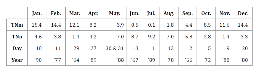
Table 4. TNm and TNn values and their date of occurrence (°C) (1991-2020).
Tabla 4. Valores de TNm y TNn y su fecha de ocurrencia (°C) (1991-2020).
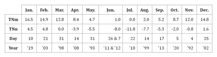
Table 5 and table 6, show TXm and TXx values and their date of occurrence for 1961-1990 and 1991-2020.
Table 5. TXm and TXx values and their date of occurrence (°C) (1961-1990).
Tabla 5. Valores de TXm y TXx y su fecha de ocurrencia (°C) (1961-1990).
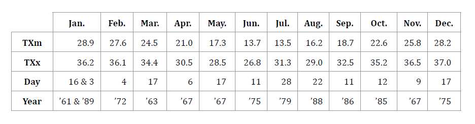
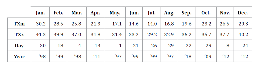
Table 6. TXm and TXx values and their date of occurrence (°C) (1991-2020).
Tabla 6. Valores de TXm y TXx y su fecha de ocurrencia (°C) (1991-2020).
Average Daily Temperature (TMm)
Annual mean air temperatures (tables 1 and 2), show that the 1991-2020 period was 0.6°C warmer than the previous 30-year period. The SD also increased in the second period by 0.2°C, implying more frequent or extremely high temperatures, as mean values have also escalated. This is confirmed by comparing TNm, TNn, TXm, and TXx values in tables 3, 4, 5 and table 6; figure 1.
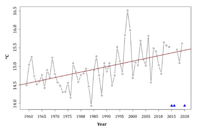
Figure 1. Sen’s slope of annual average daily temperatures (1959-2020).
Figura 1. Pendiente de Sen de las temperaturas medias diarias anuales (1959-2020).
Average daily temperatures registered a highly significant increase of 0.15°C per decade (p-value <0.00001). The greatest contribution occurred during the summer quarter (DJF) with 0.25 °C.decade-1, and the winter quarter (JJA), the lowest with 0.09°C.decade-1.
In Argentina, average increase in mean annual temperatures was approximately 0.7°C between 1961 and 2020, which gives an estimated increase of 0.12°C per decade, close to the 0.15°C per decade (1959-2020) obtained for our site. The global increase was 1°C in the same period, giving an estimate of 0.17°C per decade (1).
Average Daily Minimum Temperature (TNm)
Average daily minimum temperatures are significantly increasing at a rate of 0.12°C per decade (p-value <0.00001). All quarters had positive slopes, except for winter (JJA), whose slope was zero. The trends (°C.decade-1) were 0.22 (DJF), 0.12 (MAM), and 0.11 (SON). Other authors have also reported increased average annual temperatures in the Cuyo Region in 1960 - 2010 (3) and in the Humid Pampa Region in 1936-2019, particularly attributable to higher minimum temperatures in spring and summer (9) (figure 2).
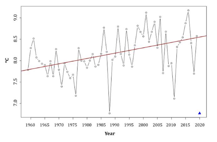
Figure 2. Sen´s slope of the annual average daily minimum temperatures (1959-2020).
Figura 2. Pendiente de Sen de las temperaturas mínimas medias diarias (1959-2020).
Minimum Monthly Value of Daily Minimum Temperature (TNn)
The “temperature of the coldest night” shows a tendency to register an increase of 0.11°C per decade (p-value = 0.37), where the greatest contribution is registered during the winter quarter (JJA) with a 0.12°C per decade increase, and the lowest during springtime (SON) with a 0.05°C per decade increase. TNn also records increases in the “humid pampas” (9), in the Cuyo region (3), and appears in the analysis of extreme temperature trends in Argentina (11) (figure 3).
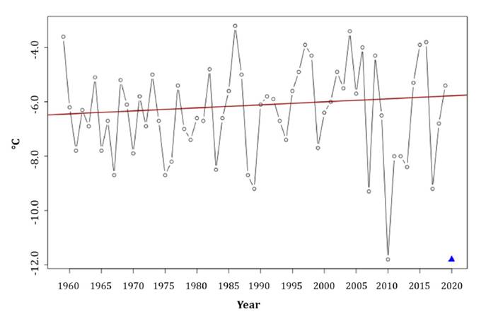
Figure 3. Sen’ s slope of the annual coldest daily minimum temperatures (1959-2020).
Figura 3. Pendiente de Sen de las temperaturas mínimas diarias absolutas (1959-2020).
Percentage of Days with Minimum Temperatures Under the 10th Percentile
The percentage of cold nights (TN10p) decreased 0.49 percentage points per decade (p-value = 0.04). The winter quarter (JJA) showed no trend, while the other quarters had values of -1.03 (DJF), -0.22 (MAM), and -0.42 (SON) (%.decade-1). In central Argentina, a lower percentage of cold nights has also been observed from October to January and in March and June (12) (figure 4).
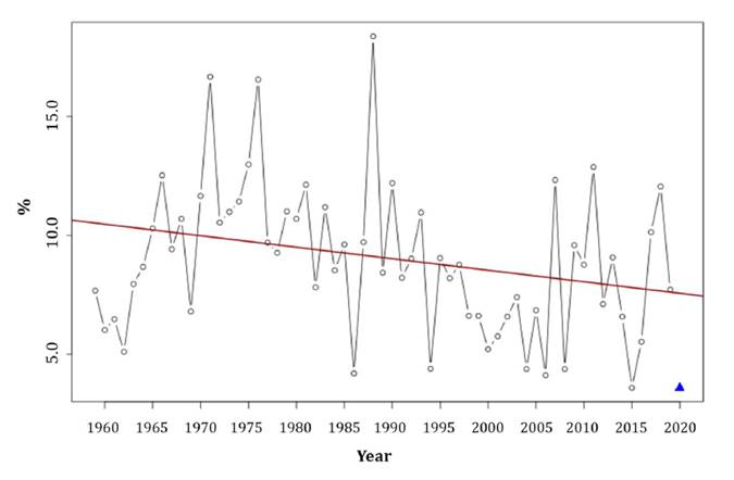
Figure 4. Sen’s slope of the annual percentage of cold nights (1959-2020).
Figura 4. Pendiente de Sen del porcentaje anual de noches frías (1959-2020).
Average Daily Maximum Temperature (TXm)
Average maximum temperatures registered a significant increase of 0.2°C per decade (p-value <0.000), with particular contribution from the spring and summer quarters with 0.21 and 0.31°C.decade-1, respectively. However, in a general provincial analysis, no significant positive trend was observed between 1997 and 2017 (8). In a more detailed analysis, only north and south Mendoza recorded significant increases of 0.5°C in 1960-2010 (3) (figure 5).
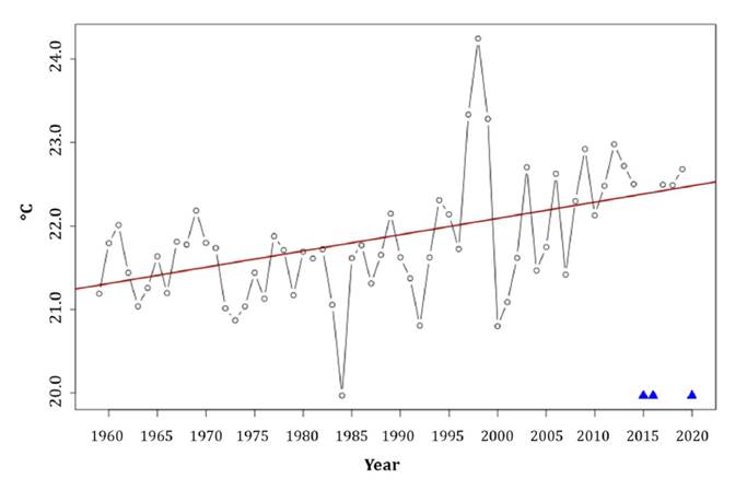
Figure 5. Sen´s slope of the annual average of daily maximum temperatures (1959-2020).
Figura 5. Pendiente de Sen temperaturas máximas medias diarias anuales (1959-2020).
Monthly Maximum Value of Daily Maximum Temperature (TXx)
Maximum temperatures of the warmest days registered a highly significant increase of 0.33°C per decade (p-value <0.000). The four quarters presented positive slopes, although the spring quarter (SON) contributed the least, with an increase of 0.24°C decade-1. Increasing maximum temperatures were also recorded in nearby areas, such as northwestern Argentina, with October having the highest frequency (2) (figure 6).
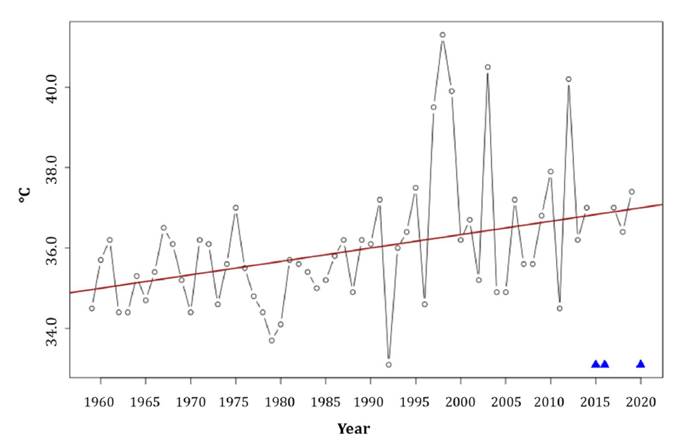
Figure 6. Sen´s slope of the annual warmest daily maximum temperatures (1959-2020).
Figura 6. Pendiente de Sen de las temperaturas máximas absolutas diarias (1959-2020).
The detected increase in both maximum and minimum temperatures suggests a growing pressure on crop water demand due to intensified evapotranspiration. This historical thermal trend provides a fundamental input for modeling future scenarios within the methodological framework of Farreras et al. (2026). Integrating these projections would allow for estimating the future evolution of the Water Footprint (WF), evaluating how increased irrigation requirements will impact water security and social welfare in the Mendocinian Northern Oasis.
Percentage of Days with Maximum Temperatures Over the 90th Percentile
The annual fraction of days with hot daytime temperatures (TX90p) rose at a rate of 1.6% per decade (p-value <0.000), with the DJF quarter contributing the most (3.10%.decade-1) compared with the JJA quarter (0.99 %.decade-1). Spring and fall show similar trends, 1.31 and 1.40%.decade-1 respectively. In central Argentina, increases in the percentage of TX90p have been recorded in March, August, and November (12), along with increasing heat waves in Mendoza (3). Between 1941 and 2000, and every 20 years, alternations of the hot extremes were observed, corresponding to an increase in the last years of the 20th century (14). Had this pattern continued, it should have decreased between 2001 and 2020; however not observed in this analysis (figure 7).
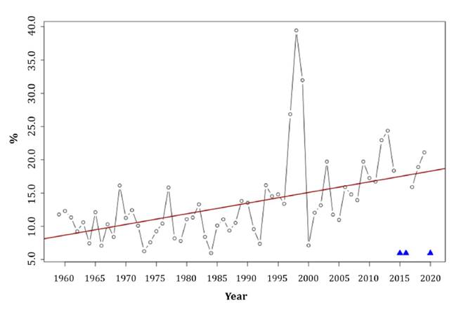
Figure 7. Sen’ s slope of the annual percentage of hot daytime temperatures (1959-2020).
Figura 7. Pendiente de Sen porcentaje de máximas mayores al percentil 90 (1959-2020).
Daily Thermal Range (DTR)
The daily thermal range increased 0.11°C per decade (p-value= 0.013), with the winter period contributing the most (0.25°C decade-1).
In 2021, the IPCC reported a declining trend for global DTR, mainly during 1960-1980 (6). In Argentina, a similar decrease was reported in the thermal amplitude due to the decreasing extremes of maximum and minimum temperatures from 1941 to 2000 (14) or given to minimum temperatures increasing more than maximum ones, particularly in central Argentina. This asymmetrical growth of maximum and mínimum temperatures would lead to reduced daily ranges, mainly due to warmer nights (2).
Nevertheless, later studies showed that the global observed DTR trend was reversed during 1980-2021, significantly growing at a rate of 0.091 ± 0.008°C per decade. The trend was dominated by a faster rate of increasing daily maximum air temperature. A 0.063 ± 0.012°C per decade global land DTR trend was reported due to a faster rate of rising daily maximum air temperature (6). This data also agrees with our observations since the growing trend of TXm is 66.6% greater than TNm (figure 2 and figure 5). Analogous results were reported in Colombia for the 1981-2020 period (10) (figure 8).
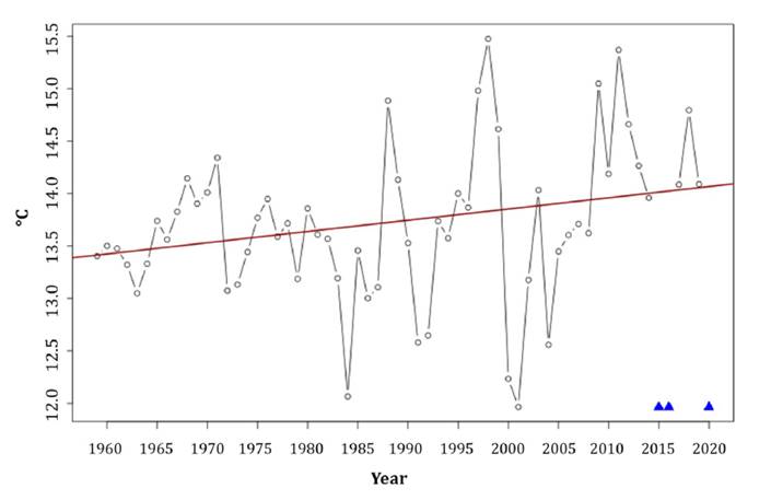
Figure 8. Sen’s slope of the mean annual daily temperature range (DTR) (1959-2020).
Figura 8. Pendiente de Sen amplitud térmica media diaria anual (DTR) (1959-2020).
Annual Accumulation of Degree Days Base 10 °C (gddgrow10)
The annual sum of the differences between average daily temperatures (TMm) and a base value of 10°C, where TMm > 10°C, measures heat accumulation to predict development rates of ectothermic organisms. In this case, we found a highly significant incremental rate of 52 Degree Days per decade (p-value <0.000) (figure 9).
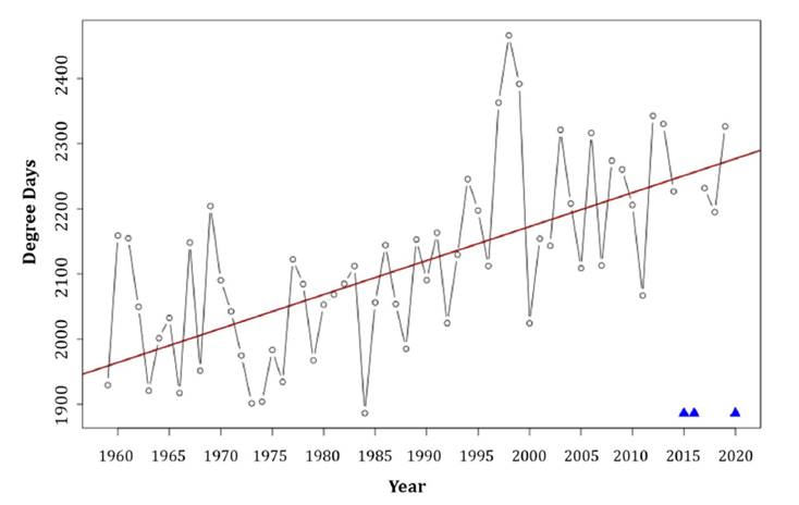
Figure 9. Sen’s slope of the annual accumulation of Degree Days base 10°C (1959-2020).
Figura 9. Pendiente de Sen de la acumulación anual de grados día base 10°C (1959-2020).
Number of Days with Frost (FD)
Based on the 1959-2019 data, the site presented an annual average of 47.3 ± 12.1 days with frosts. Figure 10 shows the monthly distribution of days with frosts. In both cases, 2020 was discarded from the analysis, given missing data for March, April, May, June, and August (figure 10).
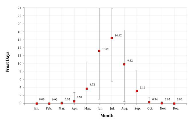
Figure 10. Distribution of days with frosts and non-parametric prediction intervals (1959-2019).
Figura 10. Distribución de días con heladas e intervalos de predicción no paramétrica (1959-2019).
No significant increase in days with meteorological frost was observed for our study site. The Sen slope was 0.024 (p-value = 0.765), and the frost regime remained practically constant during the analyzed period. However, a joint analysis for Mendoza and San Juan provinces showed a downward trend in annual frost frequency (1), as found in the humid pampas for 1981-2000 (14) (figure 11).
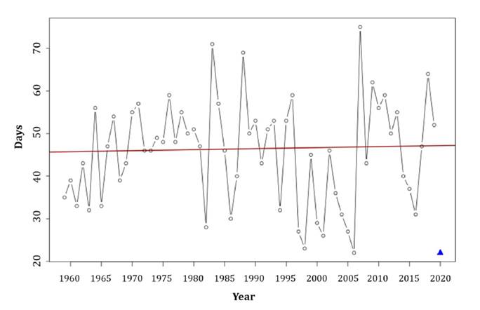
Figure 11. Sen’ s slope of days with meteorological frosts (1959-2020).
Figura 11. Pendiente de Sen de días con heladas meteorológicas (1959-2020).
Conclusions
We present the 1961-2020 trends for the main indices suggested by the WMO for global warming and climate change. Although these trends should not be extrapolated beyond the period considered, they constitute a solid comparison basis for the next climate normal (2001-2030). Our results confirm the progressive increase in temperatures observed globally. Winter, and more frequently, summer are the most affected seasons. Changing temperatura parameters are evidenced by increasing maximum and minimum temperatures, decreasing percentage of cold nights (TN10p), and increasing percentage of warmer days (TX90p).
The significantly larger availability of Degree Days based on 10°C also indicates greater energy availability, shortening cycles of ectothermic organisms as long as extreme temperatures, especially maximum temperatures, do not become stressful. Thus, impacts on growth rates of ectothermic organisms should be expected, as well as effects of extremely high temperatures on their physiology and behavior.
Trends found at our local level agree with those worldwide. Although both minimum and maximum temperatures are increasing, higher values observed in the daily thermal range are explained by a greater increase in maximum temperatures than in minimum temperatures.
1. Alabar, F.; Valdiviezo Corte, M.; Moreno, C.; Hurtado, R. 2022. Temperaturas extremas registradas en estaciones del noroeste argentino. XIX Reunión Argentina de Agrometeorología: Producción Armónica y Sustentable. Asociación Argentina de Agrometeorología. https://www.siteaada.org/_files/ugd/ cf1a17_2f530752296445dc92edabb44abeeecc.pdf
2. Aneise, A. J.; Möhle, E.; Risaro, D. B.; Schteingart, D. 2024. Cambio climático. Argendata. Fundar. https://argendata.fund.ar/topico/cambio-climatico/. Retrieved June 19th, 2025.
3. Araneo, D. 2015. Foro de Cambio Climático. Efectos del Cambio Climático en Mendoza y propuestas de adaptabilidad. UNCUYO-ONU. https://www.uncuyo.edu.ar/centroasuntosglobales/upload/foro-de-cambio-climatico-presentacion-diego-araneo.pdf
4. Commission for Climatology (CCl). 2024. Expert Team on Climate Risk and Sector-Specific Climate Indices (ETCRSCI). Climpact user guide. https://github.com/ARCCSS-extremes/climpact/blob/master/www/user_guide/Climpact_user_guide.md. Retrieved February 27th, 2024.
5. Córdoba, M.; Vallone, R.; Paccioretti, P.; Corvalán, F.; Balzarini, M. 2025. Data-driven Method for the Delimitation of Viticultural Zones: Application in the Mendoza River Oasis, Argentina. Revista de la Facultad de Ciencias Agrarias. Universidad Nacional de Cuyo. Mendoza. Argentina. 57(2): 57-68. DOI: https://doi.org/10.48162/rev.39.171
6. Di Rienzo, J. A.; Casanoves, F.; Balzarini, M.; Gonzalez, L.; Tablada, M.; Robledo, C. W. 2020. InfoStat versión 2020. Centro de Transferencia InfoStat. FCA. Universidad Nacional de Córdoba.
7. Farreras González, V. I.; Lauro, C.; Abraham, L.; Salvador, P. F. 2026. Social Welfare Effects of Water Security Improvements in Arid Regions: The Case of Mendoza, Argentina. Revista de la Facultad de Ciencias Agrarias. Universidad Nacional de Cuyo. Mendoza. Argentina. 58(1): e8916. DOI: https://doi.org/10.48162/rev.39.195
8. Huang, X.; Dunn, R. J.; Li, L. Z.; McVicar, T. R.; Azorin-Molina, C.; Zeng, Z. 2023. Increasing Global Terrestrial Diurnal Temperature Range for 1980-2021. Geophysical Research Letters, 50(e2023GL103503). doi.org/https://doi.org/10.1029/2023GL103503
9. IPCC. 2013. Annex III: Glossary [Planton, S. (ed.)]. In: Climate Change 2013: The Physical Science Basis. Contribution of Working Group I to the Fifth Assessment Report of the Intergovernmental Panel on Climate Change [Stocker, T. F., D. Qin, G.-K. Plattner, M. Tignor, S.K. Allen, J. Boschung, A. Nauels, Y. Xia, V. Bex and P.M. Midgley (eds.)]. Cambridge University Press.
10. Mulena, G. C.; Araneo, D. C. 2018. Variabilidad y tendencia de los extremos de temperatura sobre la provincia de Mendoza, Argentina. CONGREMET XIII. https://cenamet.org.ar/congremet/wp-content/uploads/2018/11/T0099_MULENA.pdf
11. Müller, G. V.; Lovino, M. A.; Sgroi, L. C. 2021. Observed and Projected Changes in Temperature and Precipitation in the Core Crop Region of the Humid Pampa, Argentina. Climate. 9(3): 40. https://doi.org/10.3390/cli9030040
12. Ruiz Murcia, J. F.; Melo Franco, J. Y.; Herrera Aponte, S. M.; Fonseca Gutiérrez, E. K.; Vega Burgos, A. 2023. Cálculo de indicadores (evidencias) de cambio climático para Colombia 1981-2020. IDEAM-METEO / 004-2023. Instituto de Hidrología, Meteorología y Estudios Ambientales. Grupo de modelamiento numérico de tiempo y clima. Grupo de gestión de datos y red meteorológica. IDEAM.
13. Rusticucci, M.; Barrucand, M. 2004. Observed trends and changes in temperature extremes over Argentina. Journal of Climate. 17(20): 4099-4107.
14. Rusticucci, M.; Barrucand, M.; Collazo, S. 2016. Temperature extremes in the Argentina central region and their monthly relationship with the mean circulation and ENSO phases. International Journal of Climatology. 37(6): 3003-3017. https://doi.org/10.1002/joc.4895
15. Sen, P. K. 1968. Estimates of the Regression Coefficient Based on Kendall’s Tau. Journal of the American Statistical Association. 63(324): 1379-1389. doi.org/10.1080/01621459.1968.10480934
16. Tencer, B.; Rusticucci, M. 2012. Analysis of interdecadal variability of temperature extreme events in Argentina applying EVT. Atmósfera. 25(4): 327-337. http://www.scielo.org.mx/scielo.php?script=sci_arttext&pid=S0187-62362012000400002&lng=es&tlng=en
17. Wang, X. L. 2008a. Accounting for autocorrelation in detecting mean-shifts in climate data series using the penalized maximal t or F test. J. Appl. Meteor. Climatol. (47): 2423-2444. doi.org/10.1175/2008JAMC1741.1
18. Wang, X. L. 2008b. Penalized maximal F-test for detecting undocumented mean-shifts without trend-change. J. Atmos. Oceanic Tech. V (3): 368-384. doi.org/10.1175/2007/JTECHA982.1
19. Wang, X. L.; Feng, Y. 2013. RHtestsV4 User Manual. Climate Research Division, Atmospheric Science and Technology Directorate. Science and Technology Branch Environment. http:// etccdi.pacificclimate.org/software.shtml
20. WMO and Green Climate Fund (GCF) Secretariats. 2022. Developing the Climate Science Information for Climate Action WMO-No. 1287. World Meteorological Organization. https://library.wmo.int/idurl/4/53280
21. World Meteorological Organization. 2017. WMO Guidelines on the Calculation of Climate Normals WMO-No. 1203. World Meteorological Organization. https:// library.wmo.int/viewer/55797/download?file=1203_en.pdf&type=pdf&navigator=1
22. World Meteorological Organization. 2020. Guidelines on Homogenization WMO-No. 1245. World Meteorological Organization. https://library.wmo.int/ idurl/4/57130
23. World Meteorological Organization. 2023. Guide to Climatological Practices WMO-No. 100. World Meteorological Organization. https://library.wmo.int/ idurl/4/60113
24. World Meteorological Organization. 2023. The Global Climate 2011-2020. A decade of accelerating climate change. WMO-No. 1338. World Meteorological Organization. https:// library.wmo.int/idurl/4/68585
25. Zwiers, F. W.; Zhang, X. 2009. Guidelines on Analysis of extremes in a changing climate in support of informed decisions for adaptation WMO/TD-No. 1500. World Meteorological Organization. https://library.wmo.int/idurl/4/48826