Rev. FCA UNCuyo | 2026 | 58(1) | ISSN 1853-8665

Natural resources and environment

https://doi.org/10.48162/rev.39.214

Predictive Modeling of Effective Electrical Conductivity for Irrigation Water in Mendoza, Argentina

Modelo predictivo de conductividad eléctrica efectiva para aguas de riego en Mendoza, Argentina

Daniela Virginia Cónsoli ^1*,

María Flavia Filippini ¹

¹ Universidad Nacional de Cuyo. Facultad de Ciencias Agrarias. Departamento de Ingeniería Agrícola. Almirante Brown 500. M5528AHB. Chacras de Coria. Mendoza. Argentina.

^* dconsoli@fca.uncu.edu.ar

Abstract

This study develops five predictive models based on regression trees to estimate the Effective Electrical Conductivity (CEE) of irrigation water in the Green Belt of Mendoza, Argentina. Using 468 water samples and physicochemical measurements from the Chachingo and Pescara canals, the models incorporate between one and six predictor variables. The most prominent model includes values of Actual Electrical Conductivity (CEA), calcium, magnesium, and bicarbonate ions, with a correlation coefficient of 0.99 and a mean absolute error of 26.5 μS cm^-1. CEE is a key indicator for assessing water quality in areas with moderately soluble salts. These models provide a cost-effective tool for identifying salinity risks in irrigation water of varying quality. Their simplicity and robustness make them suitable for Mendoza or other regions with similar conditions, supporting efficient water resource management in agriculture.

Keywords: effective electrical conductivity, irrigation water, regression tres, water quality, salinity, green belt

Resumen

Este estudio desarrolla cinco modelos predictivos basados en árboles de regresión para estimar la Conductividad Eléctrica Efectiva (CEE) del agua de riego en el Cinturón Verde de Mendoza, Argentina. Utilizando 468 muestras de agua y mediciones fisicoquímicas de los canales Chachingo y Pescara, los modelos emplean entre 1 y 6 variables predictoras. El modelo más destacado incluye valores de Conductividad Eléctrica Actual (CEA), iones calcio, magnesio y bicarbonatos, con un coeficiente de correlación de 0,99 y un error absoluto medio de 26,5 μS cm^-1. La CEE es crucial para evaluar la calidad del agua en áreas con sales de mediana solubilidad. Estos modelos permiten a productores, técnicos e investigadores realizar análisis más económicos, facilitando la identificación de riesgos salinos en aguas de calidad variable. Su simplicidad y robustez los hacen aplicables no solo en Mendoza, sino también en otras regiones con condiciones similares, contribuyendo al manejo eficiente de los recursos hídricos en la agricultura.

Palabras clave: conductividad eléctrica efectiva, agua de riego, árboles de regresión, calidad del agua, salinidad, cinturón verde

Originales: Recepción: 25/09/2025- Aceptación: 12/03/2026

Introduction

The arid province of Mendoza critically relies on the efficient management of water resources, primarily originating from snowmelt in the Andean mountain range. This water availability has enabled the development of agricultural oases that occupy only 4% of the provincial territory but concentrate 98% of the population and agro-industrial activities. Within this framework, irrigation water quality in the Northern Oasis -where the Green Belt is located- is key for the production of vegetables and fruits that supply the Mendoza Metropolitan Area and other national markets. However, the increasing water demand from agricultural, industrial, and urban sectors has exacerbated water quality problems (Zuluaga et al., 2011), driving the continuous development of strategies to promote rational use and sound management of the resource across productive sectors (Ardila & Saldarriaga, 2013).

Irrigation water systems in arid regions are characterized by strong spatial variability and environmental heterogeneity, requiring analytical approaches capable of capturing complex interactions and spatial dependence (Ciardullo et al., 2025).

Globally, agriculture is the largest consumer of freshwater and major driver of surface and groundwater degradation (FAO, 1997). In Mendoza, regional geochemical characteristics -particularly the presence of moderately soluble salts- limit the applicability of international classifications, such as the Riverside system modified by Thorne-Peterson (1954, 1996) and the FAO guidelines (Ayers & Wescot, 1987), which also inform the Ente Provincial del Agua y Saneamiento criteria (EPAS, 1995). In contrast, the classification proposed by Wainstein (1968) adapts the Riverside scheme [modified by Thorne-Peterson], incorporating Effective Electrical Conductivity (CEE), gypsum content, and the role of drainage in eliminating sodium excess (Avellaneda et al., 2004). Nevertheless, calculating CEE requires a complete physicochemical analysis, and budgetary constraints often hinder its practical use.

Defining CEE in the study area provides a more accurate interpretation of water quality, considering moderately soluble salts strongly influence water chemistry. This underscores the importance of estimating CEE using a reduced set of easily accessible, low-cost variables. We address this methodological gap with regression trees to predict CEE based on various physicochemical variables.

A decision tree is an algorithm that analyzes information and establishes associations between profiles (independent variables) and a target outcome (dependent variable) (Díaz-Martínez et al., 2021). The response may be categorical (classification trees) or continuous (regression trees). These trees generate recursive partitions through classification rules until a final classification, identifying profiles (terminal nodes) and probabilities (Cardona Hernández, 2004). These techniques offer certain advantages over other multivariate classification or prediction methods. The first advantage is their non-parametric nature, without assumptions about the distribution of predictor variables, their relationship with the response, or possible interactions. A decision tree makes optimal choices from a probabilistic perspective (Díaz-Martínez et al., 2021). Generally, the inherent logic of decision trees makes them simpler to interpret than other multivariate regression methods (Calle & Sánchez-Espigares, 2007). This methodology has proven effective in data mining, allowing segmentation and classification of large volumes of information to predict variables of interest, such as CEE. Consequently, water quality can be assessed using a limited number of physicochemical variables, facilitating resource monitoring.

In recent years, data-driven approaches integrating multiple environmental variables and machine-learning techniques have proven effective for analyzing complex agro-environmental systems, enabling the identification of key drivers and improving the interpretation of spatial variability (Córdoba et al., 2025).

This methodology offers new perspectives on water quality that might be applied in other regions with similar geochemical conditions. To date, no scientific studies have proposed methodological alternatives for estimating CEE beyond the traditional approach proposed by Wainstein (1968), based on the CEE calculation developed by Nijensohn (1961).

This study advances knowledge concerning irrigation water quality, particularly in areas requiring more tailored and accessible approaches. The predictive model of Effective Electrical Conductivity (CEE) aimed to optimize water classification in the Mendoza Green Belt and provide a practical tool to inexpensively evaluate water quality, supporting more efficient and sustainable water resource management.

Materials and Methods

The study area is located within the Mendoza Green Belt (approximate coordinates 32°53’ S - 68°42’ W), a region devoted to intensive vegetable production that includes the districts of Los Corralitos, La Primavera, Km 8, Mundo Nuevo, and Las Violetas. The area has a semi-arid climate, with scarce rainfall concentrated in summer (200-250 mm annually), extreme temperatures, and frequent winter frosts (Ramos et al., 2017). Soils have high organic matter and a shallow water table (Akil, 2020). Since the commissioning of the Potrerillos Dam in 2003, irrigation management in this area shifted from a traditional system with irregular water availability to a more controlled and efficient approach.

This study considers a prior monitoring work conducted between 1999 and 2013 by Facultad de Ciencias Agrarias (FCA) and Instituto Nacional del Agua (INA), with a large dataset for the study area (Cónsoli, 2015). During this period, water samples were collected monthly or bimonthly at fixed points in the Mendoza Green Belt, specifically in the Chachingo and Pescara canals. Samples were analyzed to determine: Actual Electrical Conductivity (CEA), pH, calcium (Ca²⁺), magnesium (Mg²⁺), sodium (Na⁺), potassium (K⁺), carbonate (CO₃ 2^-), bicarbonate (CO₃H^-), chloride (Cl^-), and sulfate (SO₄ ²^-) (Official Methods of Analysis of AOAC International, 1995). Nitrates (NO₃^-) and phosphates (PO₄ 3^-) were measured using a HACH 2010 spectrophotometer, while heavy metals such as lead (Pb), copper (Cu), cadmium (Cd), and zinc (Zn) were quantified using atomic absorption spectrophotometry. Based on these analyses, additional parameters were calculated, including Effective Electrical Conductivity (CEE), Sodium Adsorption Ratio (SAR), and the alkali coefficient (K), as established by Hardman-Miller (Avellaneda et al., 2004). Furthermore, water quality classifications were performed using the Riverside classification as modified by Thorne and Peterson (1954, 1996) and the regional classification for irrigation water proposed by Wainstein (1968).

Sampling Sites

Figure 1 shows the sampling points in the field. Each site was assigned a short name and abbreviation for easy identification.

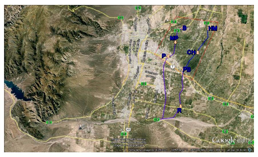
The green belt area of Mendoza is indicated in red. Source: authors’ elaboration based on Google Earth.

El área del cinturón verde de Mendoza se indica en rojo. Fuente: elaboración propia a partir de Google Earth.

Figure 1. Image of the study area with georeferenced points and a sketch of the Pescara and Chachingo channels (in blue).

Figura 1. Imagen de la zona de estudio con puntos georreferenciados y croquis de los canales Pescara y Chachingo (en azul).

The sampling points along the Chachingo Canal (or Canal Vertientes Corralitos) include: Route 60 (R), at Canal-Route 60 intersection; Puente Blanco (PB), at canal-Carril Nacional (National Drive), where water enters the Green Belt; Chachingo (CH), located in the middle section of the canal, east Corralitos; and Hijuela Montenegro (HM), final section of Chachingo Canal.

For the Pescara Canal, the Route 60 (R) point was the starting reference, since Chachingo and Pescara canals receive water from the Mendoza River within a few meters of each other. We sampled Pescara (P), at canal entrance to the Mendoza Green Belt, at canal-Carril Nacional (National Road); Matus and Pescara (MP), in the middle section of the canal, downstream from the Industrial Drainage Inspection of the Pescara Collector (Departamento General de Irrigación, DGI); and Becases (B), at the end of the canal, named after a nearby farm.

Water Characterization

Waters in the study area are generally classified as “low sodium hazard” (S1) and, according to the Riverside classification, exhibit “medium salinity” (C3), suggesting their use in soils with moderate to good permeability. In addition to selecting crops with moderate to high salt tolerance, regular leaching irrigations are recommended to prevent hazardous salt accumulation. According to Wainstein’s classification (1968), waters are generally grouped as “moderately saline” (C3) or “medium saline” (C4), with C3 waters being suitable for all crops. In salt-sensitive plants, soils without moderate to good permeability must be leached. The C4 waters are suitable for soils with lower permeability but need adequate drainage. Alternatively, moderately tolerant crops should be used with leaching irrigation.

Towards the canals’ most distant points, increased salinity and sodicity reduce irrigation suitability. These waters are classified according to Wainstein (1968) as C4 “medium saline” (15% increase in EC relative to the initial point), C5 “distinctly saline” (45%), and C6 “strongly saline” (90%), with a sodium hazard of S2 “moderate risk” (SAR exceeding 4.4 and Na⁺ values 3.9 times higher than the initial levels). In most cases, soil gypsum mitigates this hazard. However, in fine-textured soils with restricted drainage, the sodium hazard remains considerable, being most critical towards the end of the Pescara Canal, where the proportion of moderately soluble salts is lower.

Predictive Model: Regression Trees

Using data mining techniques to construct predictive models with regression trees, we obtained equations to estimate Effective Electrical Conductivity (CEE) as a function of related variables, based on Cónsoli (2015). Predictor variables were selected by degree of correlation with CEE, determination complexity, and cost. This analysis established different combinations of predictor variables varying in number (Cónsoli, 2015). This study determined correlations among quantitative measurements, descriptive and validation statistical techniques for continuous and nominal variables, and a clustering strategy to identify water quality patterns from joint measurements. Initially, Artificial Neural Networks (ANN) were applied to include missing data in the database (26 values for heavy metals and 27 for nitrates and phosphates, before 2008).

The data set used for model development consisted of 468 water samples, each with 16 analyzed parameters and others calculated from measurement results. These instances were employed in the training phase, where CEE was to be predicted. Modeling was conducted in two phases. In the first training phase, the algorithm known as M5P (Holmes et al., 1999; Quinlan, 1993; Wang & Witten, 1997), which implements a regression tree model also referred to as a “model tree”, was used to build a predictive model from the measured data. The minimum number of instances per leaf node was set at 4, with pruning and unfiltered predictions. The resulting regression tree contained intermediate nodes representing queries about attribute values, and leaf nodes containing linear models (LM) to calculate CEE.

The model validation phase included a cross-validation technique (Dietterich, 1997) with ten folds to evaluate model performance. This approach divides the dataset into 10 subsets. In each iteration, 9 subsets are used for training and 1 for validation. Metrics such as correlation coefficients, mean absolute errors, and relative squared errors assessed fit and generalization ability. Both phases used the open-source tool Waikato Environment for Knowledge Analysis (WEKA, Hall et al., 2009).

Results and Discussion

Figure 2 represents a correlation plane associating the measured variables (Cónsoli, 2015). The variables associated with component 1 (horizontal) include the alkali coefficient (K), CEA, CEE, SAR o RAS, and most of the ions present in the water. There is also variation related to component 2 (vertical), comprising the variables pH, PO₄ ^3-, and CO₃ ²⁺.

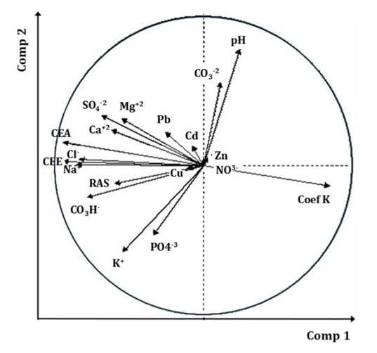
Figura 2. Plano de correlación de las variables cuantitativas.

Figure 2. Correlation plane of the quantitative variables.

The figure 2 shows that CEA, CEE, and all ions except CO₃ ²⁻ were significantly correlated. As CEA and CEE increased, Cl^- (high to near-perfect linear correlation), SO₄ ²⁻, Na⁺, Mg²⁺, Ca²⁺, and HCO₃^- (moderately high correlation), K⁺, PO₄ ³^⁻, and SAR (moderately low correlation), also tended to increase (p < 0.01). As expected from a theoretical standpoint, an inverse and statistically significant correlation was observed between CEA and the K coefficient (p < 0.01); that is, as CEA increases, K tends to decrease, requiring fewer irrigations to salinize the soil. Ions with major preponderance in waters from the study area, Cl^⁻, SO₄ ²⁻, Na⁺, Mg²⁺, Ca²⁺, and HCO₃ ^⁻, strongly influenced CEA.

Considering CEE, correlations are similar to those found with CEA, but stronger for CO₃H^⁻ (almost perfect correlation) and moderately high for Mg ²⁺. The lack of correlation between CEA or CEE and pH is corroborated.

Heavy metals, NO₃ ^⁻, and PO₄ ³⁻ show no significant relationships. Correlation between PO₄ ³⁻ and K⁺ is moderately low. CO₃ ²⁻ is the only ion not correlated with any variable, possibly due to its low presence in Mendoza waters. Statistical validation showed that the moderately low relationship between CO₃ ²⁻ and pH is the only one for this anion. The pH is inversely correlated with K⁺ (p < 0.01). The alkali coefficient (K) is negatively correlated with several variables, indicating its value decreases with increasing Cl^-, CEA, CEE (high to perfect correlation), SO₄ ²⁻, CO₃H^⁻, and Na⁺ (moderately high correlation).

These correlations (Cónsoli, 2015) are crucial to validate the use of regression trees to predict CEE from a reduced set of physicochemical variables in irrigation water. Thus, figure 2 illustrates high correlations between CEE and CEA, Cl⁻, SO₄²⁻, Na⁺, Mg²⁺, Ca²⁺, and HCO₃ ^⁻ reinforcing their selection as key predictors, excluding other variables from the model.

CEE Prediction Models

To the best of our knowledge, no previous studies have used similar methodologies to predict CEE in this area or other regions. This lack of methodological background highlights the need for innovative solutions such as regression trees, which provide accurate predictions adapted to local conditions. Our study is a pioneer, contributing knowledge on irrigation water quality and potential application in other regions with similar conditions.

To build the training set from numerical data, regression trees were developed from measurements focusing on variables that accurately predicted the numerical value of CEE in future instances. Ions showing high positive correlations with CEE were CEA, CO₃H^⁻, Cl^⁻, SO₄ ^²⁻, Ca²⁺, Mg²⁺, and Na^⁺ (Cónsoli, 2015). These variables were fundamental for the proposed models. However, SO₄ ²⁻ was excluded because its determination is costly and laborious, prioritizing those easy to measure. Based on this selection, different models were trained by progressively reducing the number of variables until an approach based exclusively on CEA to predict CEE.

Table 1 shows the five generated models (M1, M2, M3, M4, and M5) rules and equations for each case. Table 2 provides a comparative overview of the training and validation phases for each model.

Table 1. Linear Models (LM), rules and equations to predict CEE in each case.

Tabla 1. Modelos Lineales (LM) con las reglas y ecuaciones para predecir la CEE en cada caso.

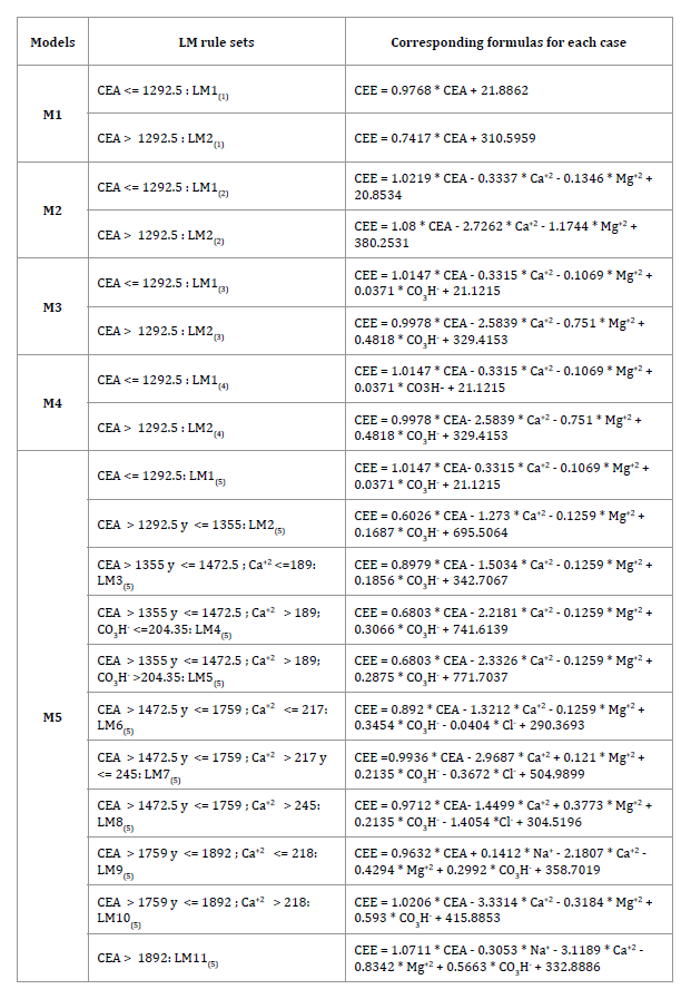
Electrical conductivities are expressed in μS cm^-1 and ion concentrations in mg L^-1. The subscript in parentheses refers to the model used.

Las conductividades eléctricas se expresan en μS cm^-1 y las concentraciones de iones en mg L^-1. El subíndice entre paréntesis hace referencia al modelo empleado.

Tabla 2. Métricas de las etapas de entrenamiento y validación, para los 5 modelos generados para predecir la Conductividad Eléctrica Efectiva (CEE).

Table 2. Metrics from the training and validation stages, for the 5 models generated to predict Effective Electrical Conductivity (CEE).

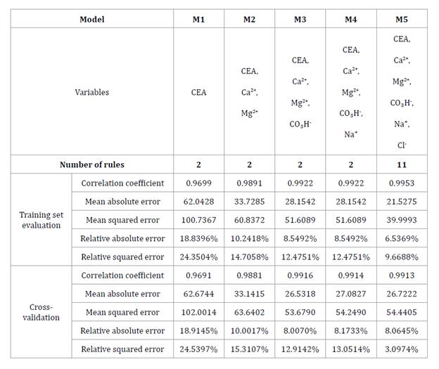
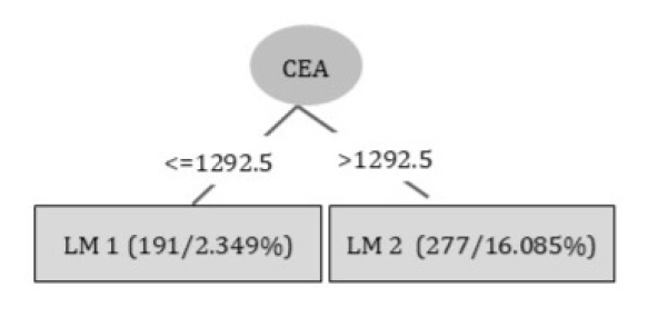
M1, M2, M3, and M4 generated identical rules: if CEA is less than or equal to 1292.5 μS cm^-1, LM1 equation is to be applied, whereas if CEA exceeds this value, LM2 equation should be used (table 1). Equations depend on variables considered in each model. Although M5 includes more variables and has a good correlation coefficient, its complexity makes it less practical.

M5 predicts CEE as a function of CEA, Ca²⁺, Mg²⁺, CO₃H⁻, Na⁺, and Cl⁻, using 11 equations depending on the values of these variables and presenting more complex rules (figure 3). A correlation coefficient of 0.99, absolute error of 21.5 μS cm^-1 in the training phase and 26.7 μS cm^-1 in validation, prove this model to be highly accurate.

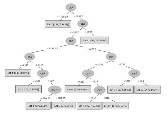
Figure 3. Regression tree of Model 5 (M5): rules of the 11 generated Linear Models (LM), support and confidence values.

Figura 3. Árbol de regresión del Modelo 5 (M5), que muestra las reglas de los 11 Modelos lineales (LM) generados, con soporte y confianza.

Subsequently, other models were generated by eliminating variables. First, Cl⁻ was excluded given its costly determination. In this way, M4 uses CEA, Ca²⁺, Mg²⁺, CO₃H^⁻, and Na⁺, and is simplified to only two equations (table 1), with a correlation coefficient of 0.99 and an absolute error of 27 μS cm-1, a very satisfactory performance.

In M3, Na⁺ was also excluded since its analysis requires a flame photometer. This model, based on CEA, Ca²⁺, Mg²⁺, and CO₃H^⁻, achieved a correlation coefficient of 0.99 and an absolute error of 26.5 μS cm-1 with only two equations, enhancing practicality without losing accuracy.

In M2, only Ca²⁺ and Mg²⁺ were used together with CEA, excluding CO₃H^⁻. This model showed a slightly lower correlation coefficient (0.989) and a higher absolute error (33 μS cm^-1).

Finally, M1 used only CEA to predict CEE, obtaining a correlation coefficient of 0.9699 and an absolute error of 62 μS cm. Although less accurate, M1 is useful when detailed ionic analyses are unavailable, allowing an acceptable estimation of CEE with minimal resources. These models can be implemented using simple software or spreadsheets to calculate CEE from basic measurements, enabling rapid and inexpensive evaluations.

Although M5 showed the best results in the training phase, cross-validation metrics of M3 were superior. This difference between training and validation suggests that M5 may have been overfit during training, limiting its generalization capacity. On the other hand, M3 is easier to apply, with only two rules or LMs compared with 11 rules in M5.

Cross-validation in this study provided a reliable assessment of the developed predictive models. This technique divides data into training and testing subsets, allowing for the identification of null overfitting. In this way, a more accurate estimate of model performance under different conditions is obtained, reducing the risk of overfitting. Cross-validation enables the identification of models with greater generalization capacity (Velásquez et al., 2013), reinforces predictive robustness, and provides greater confidence, independent of data particularities.

When the same procedure obtained a model including almost all quantified variables (CEA, Ca²⁺, Mg²⁺, CO₃H^-, Na⁺, Cl^-, pH, SAR o RAS, K⁺, CO₃ ^2-, Pb, Cu, Zn, Cd, alkali coefficient K, and classification indices such as Riverside and Wainstein, 1968), we obtained eight rules, an absolute error of 70 μS cm^-1 and a correlation coefficient of 0.98. This demonstrates that including a larger number of variables does not necessarily improve accuracy and may cause overfitting Rodriguez Murillo (2019).

Among all models, M3 stands out for sufficient accuracy and significant operational simplicity. M3 includes only the variables CEA, Ca²⁺, Mg²⁺, and CO₃H^-, significantly reducing analytical complexity without sacrificing predictive accuracy.

Compared with M4, which includes an additional variable (Na⁺), M3 maintains a similar level of accuracy while eliminating the need for a flame photometer, thus simplifying the process and reducing operational costs. Likewise, compared with M5, which incorporates up to 11 complex equations, M3 uses only two equations, easing its implementation.

Considering M2, although simpler by excluding the variable CO₃H^-, shows a higher absolute error (33 μS cm^-1) and a slightly lower correlation coefficient (0.9890), representing a clear loss of precision. M1, based exclusively on CEA, offers the greatest simplicity, but its lower accuracy limits it to preliminary estimates in contexts with severe resource constraints.

In conclusion, M3 emerges as the best option, combining accuracy and ease of application. This makes it an optimal tool for predicting CEE in various agronomic and environmental applications.

Prediction of CEE as a Function of CEA, Ca²⁺, Mg²⁺, and CO₃H- According to Model 3:

Representation of Inputs and Outputs

A: Set of attributes or input (independent) variables: CEA, Ca²⁺, Mg²⁺, and CO₃H^⁻.

V: Set of possible values of the attributes (table 3).

E: Set of 468 training instances described in terms of A, V, and a numerical value of CEE that belongs to E.

Table 3. Inputs and continuous output of Model 3 to predict Effective Electrical Conductivity (CEE).

Tabla 3. Descripción de entradas y salidas continuas del Modelo 3 para predecir la Conductividad Eléctrica Efectiva (CEE).

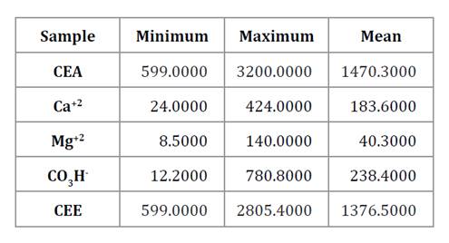
Electrical conductivities are expressed in μS cm^-1 and ion concentrations in mg L^-1.

Las conductividades eléctricas se expresan en μS cm^-1 y las concentraciones de iones en mg L^-1.

Parameters of the M5P Algorithm and Learned Model

Figure 4, shows the regression tree generated using the M5P algorithm. This model contains two rules or linear models (LMs), with a relative squared error of 12.5% in the training data. The correlation coefficient is high, reaching 0.9922.

Electrical conductivities are expressed in μS cm^-1.

Las conductividades eléctricas se expresan en μS cm^-1.

Figure 4. Regression tree of Model 3 (M3) to predict Effective Electrical Conductivity (CEE) as a function of CEA, Ca⁺², Mg⁺² and CO₃H^-, with support and confidence.

Figura 4. Árbol de regresión del Modelo 3 (M3) para predecir Conductividad Eléctrica Efectiva (CEE) en función de CEA, Ca⁺², Mg⁺² y CO₃H^-, con soporte y confianza.

The rules and equations derived from the model are as follows:

- If CEA <= 1292.5: LM1(3)

CEE = 1.0147 * CEA - 0.3315 * Ca⁺² - 0.1069 * Mg⁺² + 0.0371 * CO₃H^- + 21.1215

- If CEA > 1292.5: LM2(3)

CEE = 0.9978 * CEA - 2.5839 * Ca⁺² - 0.751 * Mg⁺² + 0.4818 * CO₃H^- + 329.4153

Validation

M3 performance shows solid predictive capacity. The correlation coefficient, which evaluates the statistical relationship between predicted and observed values, is 0.9916, indicating an excellent fit. The prediction error is 8%, considered reasonable. The mean absolute error is 26 μS cm^-1 of CEE, highly acceptable for evaluating irrigation water.

Conclusions

The predictive model of CEE, developed through regression trees, is effective, precise, and accessible for evaluating irrigation water quality in the Mendoza Green Belt.

Five models were developed, using from one to six variables (CEA). All models showed robust performance, confirming applicability in diverse scenarios. This versatility allows resource optimization while reducing costs compared to traditional analytical methods.

Model 3 stood out for simplicity and performance, predicting CEE from four key physicochemical variables: CEA, Ca²⁺, Mg²⁺, and CO₃H^⁻. The rules generated by the regression trees offer replicability and adaptability in contexts with specific geochemical characteristics.

The proposed approach improves risk interpretation in irrigation waters containing salts of medium solubility, as it is adapted to local geochemical conditions and overcomes limitations of international classification systems. This methodology provides practical alternatives, contributing to the sustainable and efficient management of water resources in Mendoza and similar regions.

These simple equations reduce analytical costs and facilitate frequent monitoring, reserving detailed ionic analyses for particular situations. Future research should focus on comparative studies to evaluate model performance in varied contexts and on refining predictor variables according to local conditions. Expanding the dataset to other regions will also help validate model adaptability, ensuring broader applicability in agricultural water management.

References

Akil, N. N. (2020). Zonificación del cinturón verde de Mendoza en base a las funciones ecosistémicas. Tesina de grado. Universidad Nacional de Cuyo. Facultad de Ciencias Agrarias. Biblioteca Digital UNCUYO. https://bdigital.uncu.edu.ar/15559

Ardila, A. N. & Saldarriaga, J. (2013) Formulación de un índice global de calidad de aguas residuales para riego. Av. Cien. Ing., 4(3), 11-26.

Avellaneda, M.; Bermejillo, A.; Mastrantonio L. E. (2004). Aguas de riego calidad y evaluación de su factibilidad de uso. EDIUNC.

Ayers, R. S. & Westcot, D. W. (1987). La calidad del agua en la Agricultura. Serie FAO Riego y Drenaje 29(1).

Calle, M. L. & Sánchez-Espigares, J. A. (2007). Árboles de clasificación y regresión en la investigación Biomédica. Medicina Clínica, 129(18), 702-706. https://doi.org/10.1157/13112516

Cardona Hernández, P. A. (2004). Aplicación de árboles de decisión en modelos de riesgo crediticio. Revista Colombiana de Estadística, 27(2), 139-151. https://revistas.unal.edu. co/index.php/estad/article/view/28808

Ciardullo, V. F.; Gennari, A. J. (2025). Agricultural Land Valuation-Hedonic Pricing and Geostatistical Advances: A State-of-the-Art Review. Revista de la Facultad de Ciencias Agrarias. Universidad Nacional de Cuyo. 57(2): 224-236. https://doi.org/10.48162/rev.39.185

Cónsoli, D. V. (2015). Evolución de la contaminación del agua de riego y clasificación de su calidad dentro del cinturón verde de Mendoza. Tesis de maestría no publicada. Maestría en Riego y Drenaje. Universidad Nacional de Cuyo.

Córdoba, M.; Vallone, R.; Paccioretti, P.; Corvalán, F.; Balzarini, M. (2025). Data-driven Method for the Delimitation of Viticultural Zones: Application in the Mendoza River Oasis, Argentina. Revista de la Facultad de Ciencias Agrarias. Universidad Nacional de Cuyo. 57(2): 57-68. DOI: https://doi.org/10.48162/rev.39.171

Díaz-Martínez, M. A., Ahumada-Cervantes, M. de los A., & Melo-Morín, J. P. (2021). Árboles de decisión como metodología para determinar el rendimiento académico en educación superior. Revista Lasallista de Investigación, 18(2), 94-104. https://revistas.unilasallista.edu.co/index.php/rldi/article/view/2724

Dietterich, T. G. (1997). Machine-learning research. AI Magazine, 18(4), 97.

Ente Provincial del Agua y Saneamiento (EPAS). (1995). Normas de calidad de aguas. Documento preliminar. Mendoza. Argentina.

FAO. (1997). Lucha contra la contaminación agrícola de los recursos hídricos. Estudio FAO Riego y Drenaje. 55 p. Por Ongley, E. D. GEMS/Water Collaborating Centre Canadá Centre for Inland Waters. http://www.fao.org/docrep/w2598s/w2598s00.htm#Contents

Hall, M., Frank, E., Holmes, G., Pfahringer, B., Reutemann, P., & Witten, I. H. (2009). The WEKA Data Mining Software: An Update. ACM SIGKDD Explorations Newsletter, 11(1). Recuperado de https://www. kdd.org/exploration_files/p2V11n1.pdf

Holmes, G., Hall, M., Frank, E. (1999). Generating Rule Sets from Model Trees. In: Foo, N. (eds) Advanced Topics in Artificial Intelligence (AI 1999). Lecture Notes in Computer Science, vol 1747. Springer, Berlin, Heidelberg. https://doi.org/10.1007/3-540-46695-9_1

Nijensohn, L. (1961). Calidad de aguas de riego (Capítulo 14). En Primer curso nacional de manejo de riego: Riego y drenaje. Mendoza, Argentina.

Official Methods of Analysis of AOAC International. (1995). 16 th Edition. Volumen I.

Quinlan, J. R. (1993). C4.5: Programs for Machine Learning. Morgan Kaufmann. Quinlan, J. R.

 Ramos, R. A., Bottesi, M. C., & Quinteros, J. R. (2017). Estimación del avance urbano sobre la interfase urbano-rural del oasis norte de la provincia de Mendoza. INTA. https://repositorio.inta.gob.ar/xmlui/handle/20.500.12123/43

Rodríguez Murillo, N. A. (2019). Análisis de validación cruzada bajo diferentes condiciones de ruido. Tesis de Maestría en Ingeniería Industrial. Tecnológico Nacional de México. 84 p.

Thorne, D. W., & Peterson, H. B. (1954). Técnica de Riego (Versión Española, 1963). México.

Thorne. D. W. & Peterson H. B. (1996). Técnica de Riego Fertilidad y Explotación de los Suelos. Editorial Continental.

Velásquez, J. D., Fonnegra R., Y., & Villa G., F. A. (2013). Pronóstico de series de tiempo con redes neuronales regularizadas y validación cruzada. Revista Vínculos, 10(1), 267-279. https://doi.org/10.14483/2322939X.4702

Wainstein, P. (1968). Clasificación de las aguas de riego de Mendoza. Informes Científicos y Técnicos N°15. Instituto de Suelos y Riego.

Wang, Y., & Witten, I. (1997). Induction of model trees for predicting continuous classes. In Proceedings of the Poster Papers of the ECML. 128-137.

Zuluaga, J. M., Drovandi, A. A., Bermejillo, A. I., Filippini, M. F., Cónsoli, D. V., Salcedo, C. E., Valdes, A. E., & Morsucci, A. L. (2011). Diagnóstico de la calidad del recurso hídrico en el cinturón verde de Mendoza, Argentina. XVI Congreso Nacional de Irrigación. Asociación Nacional de Especialistas en Irrigación. Culiacán.